Intro to Artificial Neural Networks¶

Perceptron and Feed-forward Networks
Optimzation, the Loss, and Backpropagation
Categories of Deep Learning
Survey of Common Types of ANN

Perceptron and Feed-forward Networks¶

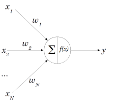
The simplest form of the ANN is the perceptron. One single unit that performs an operation on inputs and returns a single output. Here the $w_x$'s are called the weights or sometimes the parameters.

$$ \large f(w_1 x_1 + w_2 x_2 + ... + w_N x_N + b) = f\left(b + \sum_{i=1}^{N} w_i x_i \right) = y $$

$f(x)$ is called the activation function and $b$ is the bias. In principal $f$ could be anything but is typically some non-linear function.

Two Layer Perceptron¶

We can stack these perceptrons together to introduce more parameters and more non-linear behavior

$$ \large f\left(b + \sum_{i=1}^{N} w_{i} h_i(x) \right) = y $$

where $h_i(x)$ can be another set of perceptrons like in the previous slides.

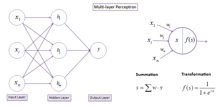
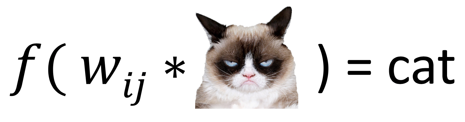
Notice that our definition of a perceptron is the same as matrix multiplication. From before we had:

$$ \large f\left(b_i + \sum_{i=1}^{N} w_{ij} x_i \right) = y_i $$
Now as matrices:
$$ \large W = \begin{bmatrix} w_{11} & w_{12} & \dots \\ \vdots & \ddots & \\ w_{i1} & & w_{ij} \\ \end{bmatrix} ;\quad X = \begin{bmatrix} x_1 \\ x_2 \\ \vdots \\ x_i \end{bmatrix} \quad \quad f\left(B + WX\right) = Y $$

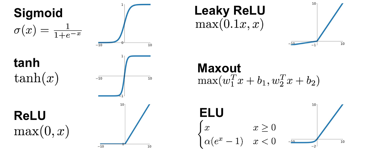
Activation Functions¶

The $f(x)$ we used earlier introduces non-linearity into the perceptron. Without non-linearities a multilayer perceptron would reduce to a single layer perceptron through a simple redefinition of parameters (the $w$s).

Cool. So What?¶

You can imagine that there exists a set of parameters W, the input of "cat" will return a value corresponding to the classification "cat".¶

Optimization, the Loss, and Backpropagation¶

Can we find the parameters $w_{ij}$ such that for an input $x$ we get the answer we want $y$?¶

This seems like a simple optimization problem. Find the $w_{ij}$ that minimize (insert thing to minimize here).

But what do we minimize? How do we find where that thing is a minimum?

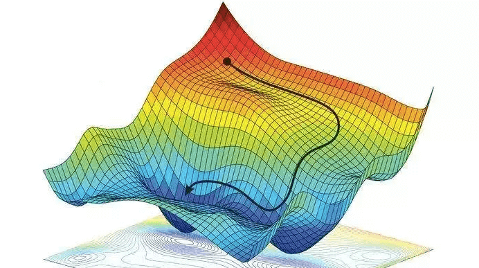
To find the bottom we can simply take a series of small steps "downhill".

The Loss¶

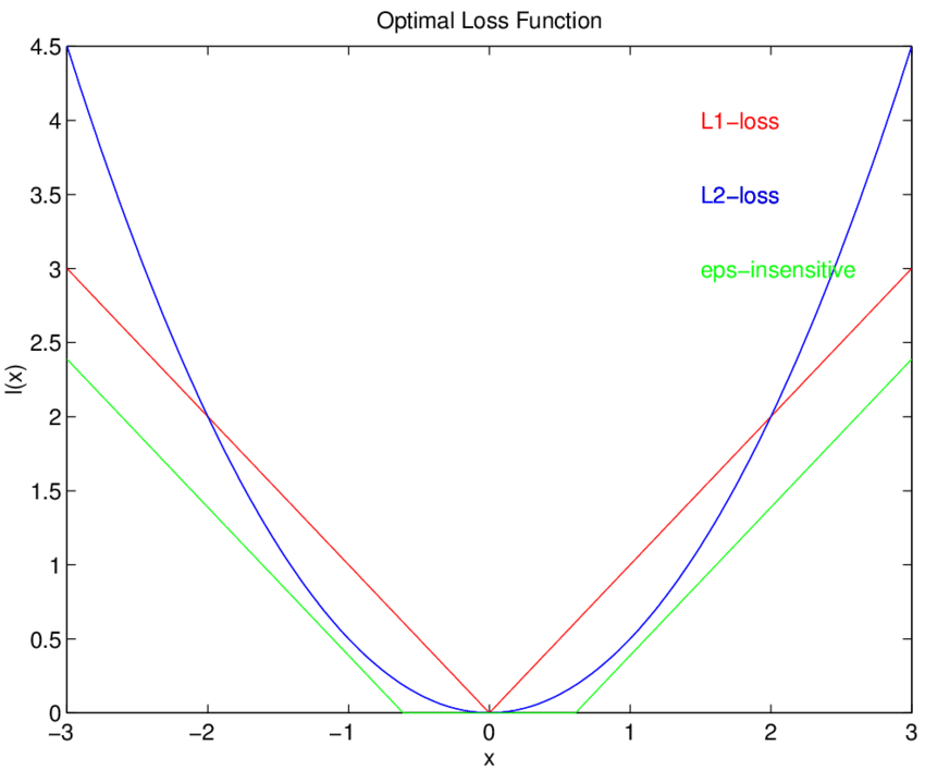
The thing to minimize we call the loss or loss function. It is simply a measure of distance between what the output of our network is and what we think it should be for a given input.

The simplest loss function you could have is the Mean Absolute Error (MAE)

$$ \Large MAE = |y-\hat{y}| $$

Here $y$ is the "target" or what we want the network to output, and $\hat{y}$ is the actual output of the network.

$$ \Large L1 = | y - \hat y | $$ $$ \Large L2 = (y - \hat y)^2 $$ $$ \Large L_{\epsilon} = \begin{cases} |y - \hat y| & \text{if $|y- \hat y| < \epsilon$} \\ 0 & \text{otherwise} \end{cases} $$

Now we just need to iteratively take steps towards the bottom of the loss.¶

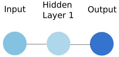
This is done by calculating the gradient at your current point then taking a step in the direction of the steepest slope. Lets consider a two layer perceptron with a single input and output.

$$ \large h(x) = f(b_1 + w_1 x) $$

is the value of the hidden unit, and

$$ \large \hat{y} = f( b_2 + w_2 h(x)) $$

is the value of the output.

The update rule for our weights is,

$$ \large w_{t+1} = w_t - \epsilon \frac{\partial L}{\partial w_t}; \space \space b_{t+1} = b_t - \epsilon \frac{ \partial L }{ \partial b_t} $$

Where $L$ is our loss function. So we need to find the gradients of the loss with respect to the parameters of the network. For a one layer network this is easy, but for deeper networks we can use the chain rule.

$$ \large \frac{\partial L}{\partial w_2} = \frac{\partial L}{\partial y} \frac{\partial y}{\partial z_2} \frac{\partial z_2}{\partial w_2} $$

where we have set $\large z_2 = b_2 + w_2 h(x)$

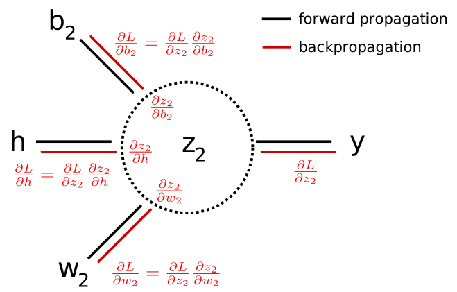
Now we simply have to take a step in the direction of the gradient...

$$ \Large w_{t+1} = w_t - step $$

... then do it again.

These are all the components needed to train a neural network¶

Linear combination of weights
Non-linear activation function
Derivatives of Loss function with respect to all parameters

Note: The way computers calculate derivates is through a process called Auto-differentiation. It uses the chain rule to split the derivative up into smaller parts until it can evaluate a math primative. This is very similar to what we want to do with backpropagation.

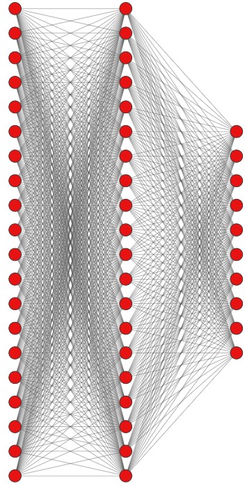
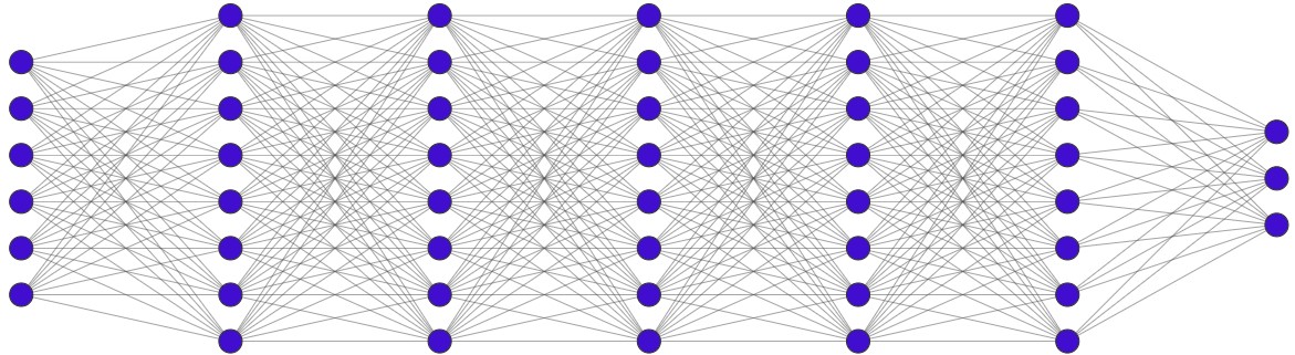
Network Width and Depth¶

Categories of Deep Learning¶

Supervised Learning¶

Data is labeled with the outcome you would like the network to reproduce.

Unsupervised Learning¶

Data has no labels. Network has to figure things out on its own.

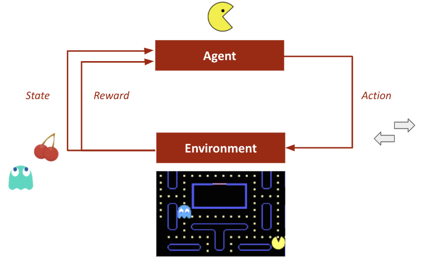
Reinforcement Learning¶

Network takes the role of an Agent which can take actions and Observe their effects on an Environment. The agent learns to take actions that maximise a desired outcome by trying to gain the most Reward.

Survey of Common Types of ANNs¶

Feed Forward Network¶

Any combination of preceptrons arranged in layers.

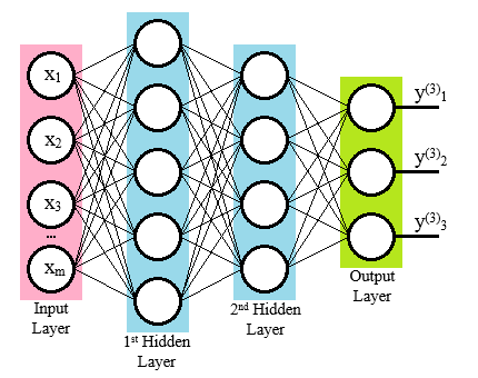
Common uses are classification and regression.

Regression Example¶

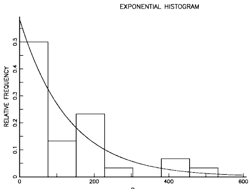
Maybe we want to find the decay parameter in the function $y=e^{-\frac{x}{\sigma}}$. In this case the input could be the $y$ value in each $x$ bin with the goal of predicting. Then the output would be our prediction of the parameter $\hat \sigma$.

Convolutional Neural Network (CNN)¶

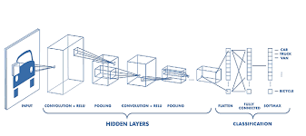
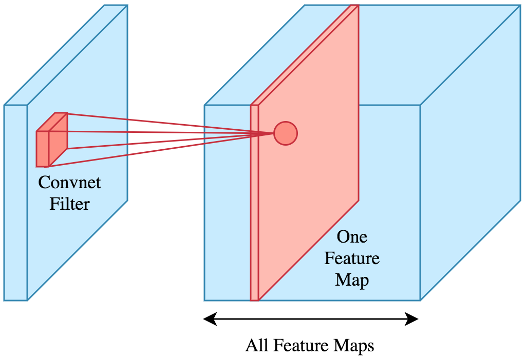
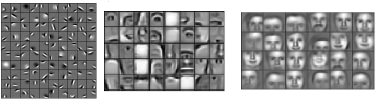
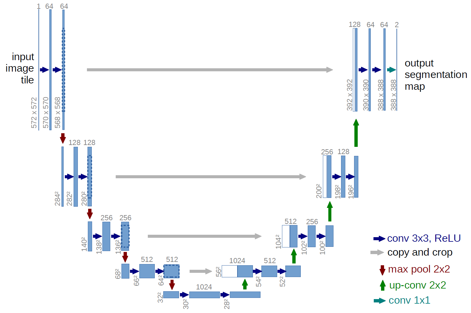
CNNs have their weights arranged into "filters". This makes them preserve spatial nature of the inputs. The easiest way to see how this works is to look at an example:

Image Kernels

Every filter is passed over the image to produce a feature map.¶

The next layer then passes a new set of filters over the feature maps.¶

U-Net CNN Architecture¶

Recurrent Neural Networks¶

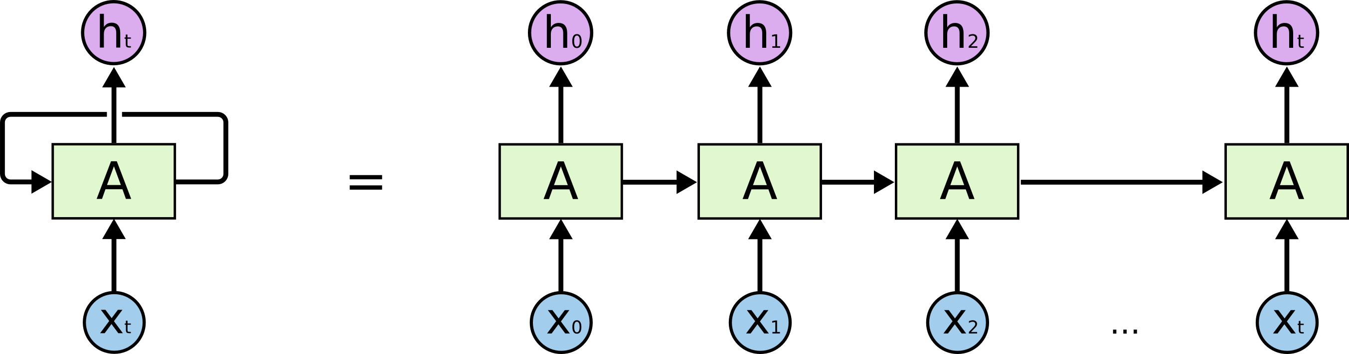
The output of the node (the hidden state) is concatenated with the next input. This recurrence allows the network to learn patterns in sequences of data.

Commonly used in NLP to generate sentences or translate from one language to another.

Encoder-Decoder RNNs¶

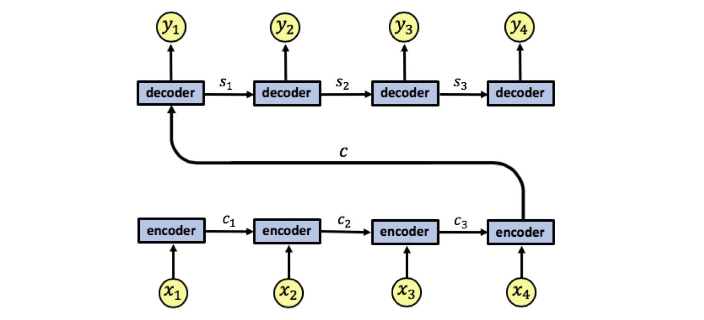
A common structure for a recurrent network is the Encoder-Decoder type model. This is where the RNN is split into two parts. The full input is passed to the decoder, then a single hidden state is passed to the decoder which generates the outputs.

Predictive NDVI¶

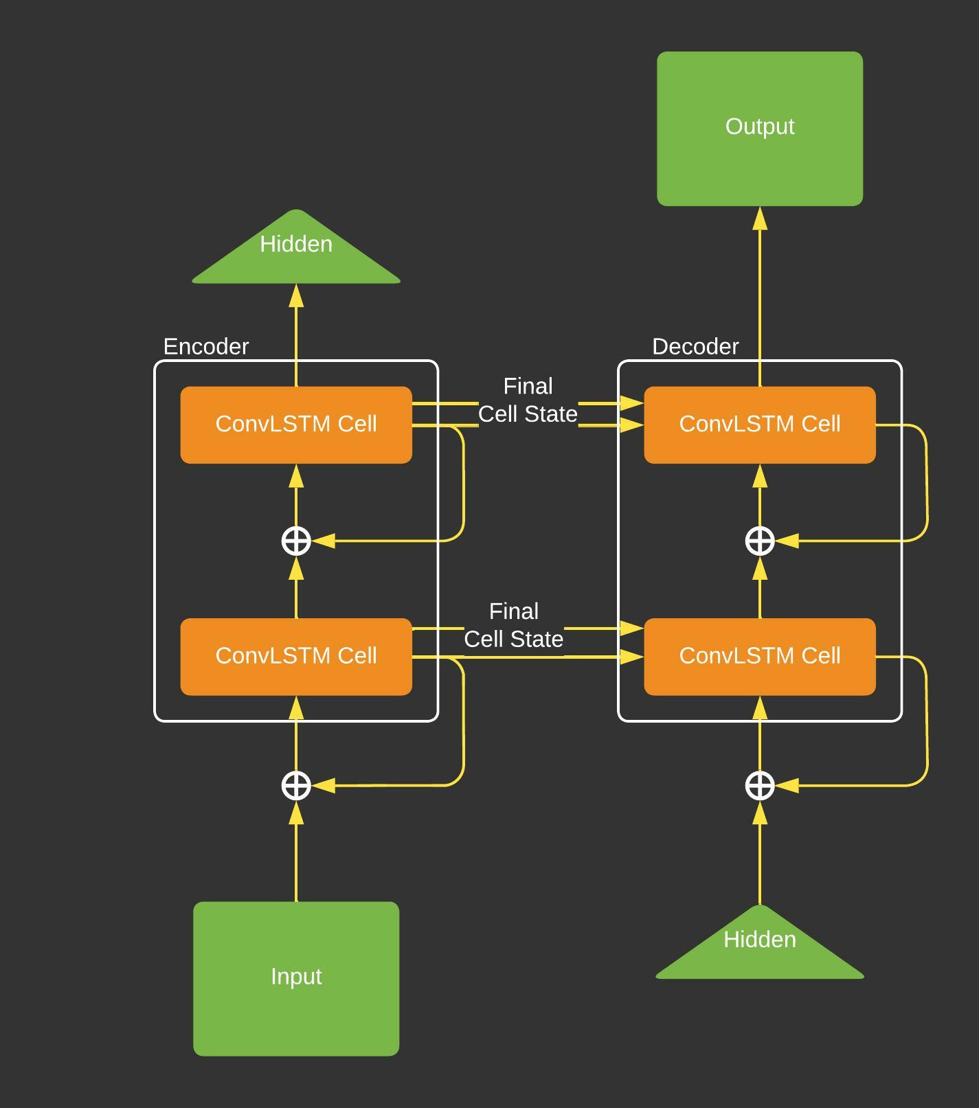
Our predictive NDVI model is an Encoder-Decoder model that uses convultional LSTMs as the network. The input is a time stack of imagery separated by 7 days.

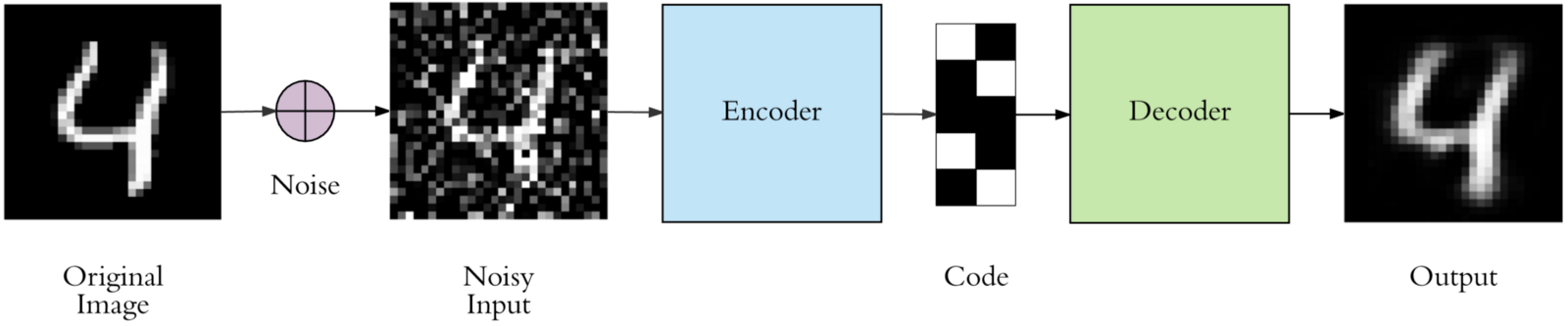
Autoencoders¶

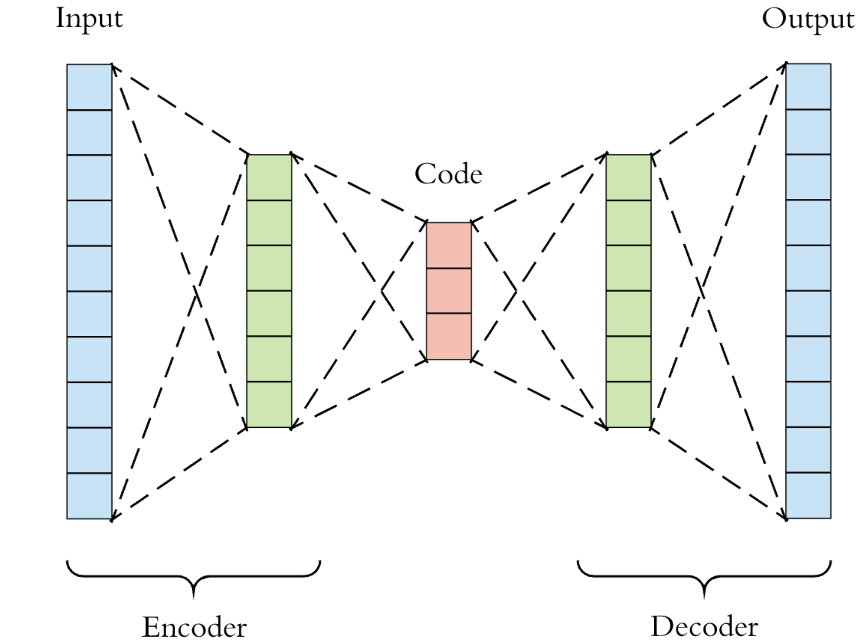
Unsupervised learning - The inputs are used as the labels.

Can be used as a learned compression for a specific type of data. Can be used as an anomoly detector by selecting inputs that have a large reconstruction error.

There are a ton of variations on autoencoders.